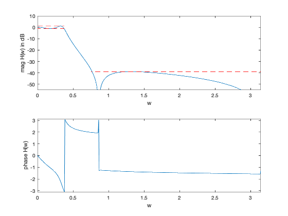
% "Linear Programming Design of IIR Digital Filters with Arbitrary
%  Magnitude Functions" by L.R. Rabiner, N.Y. Graham, and H.D. Helms
% (figures are generated)
%
% Designs a lowpass IIR filter using spectral factorization method where we:
% - minimize maximum stopband attenuation
% - have a constraint on the maximum passband ripple
%
%   minimize   max |H(w)|                      for w in the stopband
%       s.t.   1/delta <= |H(w)| <= delta      for w in the passband
%
% where we now have a rational frequency response function:
%
%   H(w) = sum_{m=0}^{M-1} b_m exp{-jwm} / sum_{n=1}^{N-1} a_n exp{-jwn}
%
% We change variables via spectral factorization method and get:
%
%   minimize   max R(w)                        for w in the stopband
%       s.t.   (1/delta)^2 <= R(w) <= delta^2  for w in the passband
%              R(w) >= 0                       for all w
%
% where R(w) is the squared magnited of the frequency response
% (and the Fourier transform of the autocorrelation coefficients r).
% We represent R(w) = N_hat(w)/D_hat(w), where now R(w) is a rational
% function since we deal with IIR filter (see the reference paper).
%
% Variables are coeffients of the numerator, denoted as c, and
% denominator, denoted as d. delta is the allowed passband ripple.
% This is a quasiconvex problem and can be solved using bisection.
%
% Written for CVX by Almir Mutapcic 02/02/06

%*********************************************************************
% user's filter specs (for a low-pass filter example)
%*********************************************************************
% number of coefficients for the IIR filter (including the zeroth one)
% (also without loss of generality we can assume that d_0 = 1, which
%  is the zeroth coefficient of the autocorrelation denominator)
M = 4; % nominator
N = 4; % denominator

wpass = 0.12*pi;   % end of the passband
wstop = 0.24*pi;   % start of the stopband
delta = 1;         % maximum passband ripple in dB (+/- around 0 dB)

%*********************************************************************
% create optimization parameters
%*********************************************************************
% rule-of-thumb discretization (from Cheney's Approx. Theory book)
sample_order = 30;
m = 15*(sample_order);
w = linspace(0,pi,m)'; % omega

% A's are matrices used to compute the power spectrum
Anum = [ones(m,1) 2*cos(kron(w,[1:M-1]))];
Aden = [ones(m,1) 2*cos(kron(w,[1:N-1]))];

% passband 0 <= w <= w_pass
ind = find((0 <= w) & (w <= wpass));    % passband
Ap_num  = Anum(ind,:);
Ap_den  = Aden(ind,:);

% transition band is not constrained (w_pass <= w <= w_stop)

% stopband (w_stop <= w)
ind = find((wstop <= w) & (w <= pi));   % stopband
As_num  = Anum(ind,:);
As_den  = Aden(ind,:);

%********************************************************************
% optimization
%********************************************************************

% use bisection (on the log of vars) to solve for the min stopband atten
Us_top = 1e-0; % 0 dB
Us_bot = 1e-6; % -60 dB (in original variables)

while( 20*log10(Us_top/Us_bot) > 1)
  % try to find a feasible design for given specs
  Us_cur = sqrt(Us_top*Us_bot);

  % formulate and solve the magnitude design problem
  cvx_begin quiet
    variable c(M,1)
    variable d(N-1,1)

    % feasibility problem
    % passband constraints
    (Ap_num*c) <= (10^(+delta/20))^2*(Ap_den*[1;d]); % upper constr
    (Ap_num*c) >= (10^(-delta/20))^2*(Ap_den*[1;d]); % lower constr
    % stopband constraint
    (As_num*c) <= (Us_cur)*(As_den*[1;d]); % upper constr
    % nonnegative-real constraint
    Anum*c >= 0;
    Aden*[1;d] >= 0;
  cvx_end

  % bisection
  if ~any(isnan(c)) % feasible
    fprintf(1,'Problem is feasible for stopband atten = %3.2f dB\n', ...
               10*log10(Us_cur));
    Us_top = Us_cur;
    b = spectral_fact(c);
    a = spectral_fact([1;d]);
  else % not feasible
    fprintf(1,'Problem not feasible for stopband atten = %3.2f dB\n', ...
               10*log10(Us_cur));
    Us_bot = Us_cur;
  end
end

% display the max attenuation in the stopband (convert to original vars)
fprintf(1,'\nOptimum min stopband atten is between %3.2f and %3.2f dB.\n',...
        10*log10(Us_bot),10*log10(Us_top));
disp('Optimal IIR filter coefficients are: ')
disp('Numerator: '), b
disp('Denominator: '), a

%*********************************************************************
% plotting routines
%*********************************************************************
% frequency response of the designed filter, where j = sqrt(-1)
H = ([exp(-j*kron(w,[0:M-1]))]*b)./([exp(-j*kron(w,[0:N-1]))]*a);

% magnitude plot
figure(1)
subplot(2,1,1)
plot(w,20*log10(abs(H)), ...
     [0 wpass],[delta delta],'r--', ...
     [0 wpass],[-delta -delta],'r--', ...
     [wstop pi],[10*log10(Us_top) 10*log10(Us_top)],'r--')
xlabel('w')
ylabel('mag H(w) in dB')
axis([0 pi -55 10]);

% phase plot
subplot(2,1,2)
plot(w,angle(H))
axis([0,pi,-pi,pi])
xlabel('w'), ylabel('phase H(w)')
Problem is feasible for stopband atten = -30.00 dB
Problem not feasible for stopband atten = -45.00 dB
Problem is feasible for stopband atten = -37.50 dB
Problem not feasible for stopband atten = -41.25 dB
Problem not feasible for stopband atten = -39.38 dB
Problem is feasible for stopband atten = -38.44 dB
Problem is feasible for stopband atten = -38.91 dB

Optimum min stopband atten is between -39.38 and -38.91 dB.
Optimal IIR filter coefficients are:
Numerator:

b =

    0.0036
   -0.0011
   -0.0011
    0.0035

Denominator:

a =

    0.2672
   -0.6977
    0.6343
   -0.1990