Cs = [ ...
0, 0 ; ...
1.2, 2.4 ; ...
-3, +3 ; ...
-4, 0 ; ...
-1.6, -3.2 ; ...
1.84615384615385, -2.76923076923077 ; ...
2.35294117647059, 0.58823529411765 ];
Cmax = max(max(abs(Cs))) * 1.25;
clf
Cx = Cs( :, 1 );
Cy = Cs( :, 2 );
m = length( Cx );
Cs = Cs';
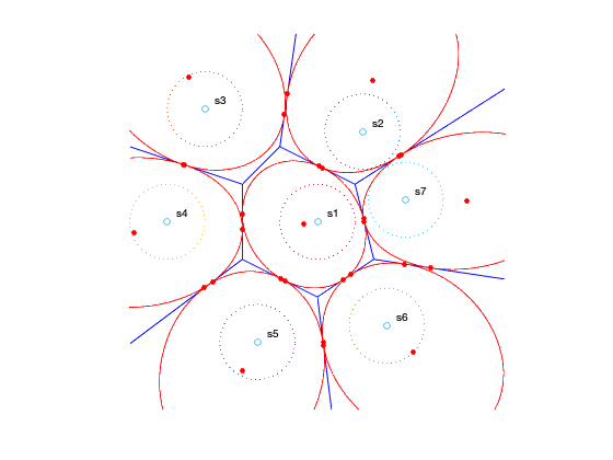
[ Vx, Vy ] = voronoi( Cx, Cy );
plot( Vx, Vy, 'b-', Cx, Cy, 'o' );
axis equal
axis( Cmax * [ -1, 1, -1, 1 ] );
axis off
hold on
noangles = 200;
angles = linspace( 0, 2 * pi, noangles );
crcpts = [ cos(angles) ; sin(angles) ];
for i=1 : m,
text( Cx(i)+0.25, Cy(i)+0.25, [ 's', int2str(i) ] );
ellipse = [ cos(angles) ; sin(angles) ] + Cs(:,i) * ones(1,noangles);
plot( ellipse(1,:), ellipse(2,:), ':' );
end;
m = size( Cs, 2 );
tri = delaunay( Cx, Cy );
ee = sparse( tri, tri( :, [ 3, 1, 2 ] ), 1, m, m );
ee = ee + ee';
for k = 1 : m,
v2 = find( ee( :, k ) );
pk = Cs( :, v2 );
qk = Cs( :, k ) * ones( 1, length( v2 ) );
Ak = pk - qk;
bk = 0.5 * sum( Ak .* Ak, 1 );
As{k} = Ak';
bs{k} = bk';
end
ints = 1 : m;
for i = ints( : ).',
[ cd_cheb, P, q, r, X, lambda ] = cheb( As{i}, bs{i}, eye(2) );
ellipse = sqrt(1-r+q'*(P\q)) * P^(-1/2) * crcpts + ...
(-P\q + Cs(:,i)) * ones(1,noangles);
plot( ellipse(1,:), ellipse(2,:), 'r-' );
dots = plot( X(1,:)+Cx(i), X(2,:)+Cy(i), 'ro' );
set( dots, 'MarkerFaceColor', 'red' );
set( dots, 'MarkerSize', 4 );
end
hold off
nsigma = 500;
sigmas = linspace( 0.001, 6.0, nsigma )';
cd_cheb = zeros( nsigma, m );
fprintf( 'Computing lower bounds' );
ints = 1 : m;
for i = ints( : ).',
for k = 1 : nsigma,
cd_cheb(k,i) = cheb( As{i}, bs{i}, sigmas(k) * eye(2) );
end;
if rem( k, 10 ) == 0,
fprintf( '.' );
end
end;
fprintf( 'done.\n' );
figure(2)
mc = size( cd_cheb, 2 );
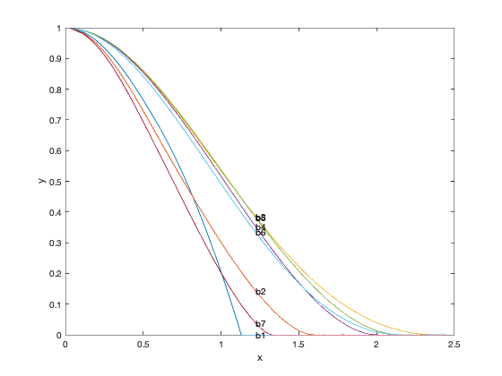
plot(sqrt(sigmas(:,ones(1,mc))), cd_cheb);
for i = 1 : mc,
text( sqrt(sigmas(nsigma/4)), cd_cheb(nsigma/4,i), ['b',int2str(i)] );
end;
xlabel('x');
ylabel('y');
axis( [ 0, 2.5, 0, 1 ] );
nsigma = 50;
sigmas = linspace( 0.1, 0.5, nsigma );
cd1 = zeros( 1, nsigma );
mc1 = zeros( 1, nsigma );
cher1 = zeros( m-1, nsigma );
fprintf( 'Computing lower bounds and Monte Carlo sims' );
for i = 1 : nsigma,
Sigma = sigmas(i)^2 * eye(2);
cd1(i) = cheb( As{1}, bs{1}, Sigma );
mc1(i) = montecarlo( As{1}, bs{1}, Sigma, 10000 );
if rem( i, 5 ) == 0,
fprintf( '.' );
end
end
fprintf( 'done.\nComputing upper bounds' );
for j = 2 : m,
A = As{j};
b = bs{j} - A * ( Cs(:,1) - Cs(:,j) );
for i = 1 : nsigma,
cher1( j - 1, i ) = cher( A, b, sigmas(i)^2*eye(2) );
end
fprintf( '.' );
end;
fprintf( 'done.\n' );
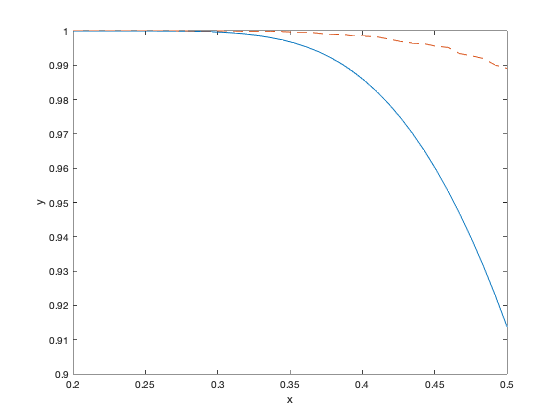
cher1 = max( 1 - sum( cher1 ), 0 );
figure(4)
plot( sigmas, cher1, '-', sigmas, mc1, '--' );
axis( [ 0.2 0.5 0.9 1 ] );
xlabel( 'x' );
ylabel( 'y' );
Computing lower bounds.......done.
Computing lower bounds and Monte Carlo sims..........done.
Computing upper bounds......done.