% Section 6.5.3
% Boyd & Vandenberghe "Convex Optimization"
% Original by Lieven Vandenberghe
% Adapted for CVX by Joelle Skaf - 10/03/05
% (a figure is generated)
%
% Given data u_1,...,u_m and v_1,...,v_m in R, the goal is to fit to the
% data a polynomial of the form
% p(u) = x_1 + x_2*u + ... + x_n*u^{n-1}
% i.e. solve the problem:  minimize ||Ax - v||
% where A is the Vandermonde matrix s.t. Aij = u_i^{j-1}
% Two cases are considered: L2-norm and Linfty-norm

% Input data
n=6;
m=40;
randn('state',0);
% generate 50 ponts ui, vi
u = linspace(-1,1,m);
v = 1./(5+40*u.^2) + 0.1*u.^3 + 0.01*randn(1,m);


% LS fit polynomial x_1 + x_2*u + ... + x_n*u^(n-1) to (ui,vi)
fprintf(1,'Computing optimal polynomial in the case of L2-norm...');

A = vander(u');
A = A(:,m-n+[1:n]);     % last n columns of A
x = A\(v');             % coefficients of the polynomial in the following
                        % order: x = [x_n x_(n-1) ... x_2 x_1]'

fprintf(1,'Done! \n');

% L-infty fit
fprintf(1,'Computing optimal polynomial in the case of Linfty-norm...');

cvx_begin quiet
    variable x1(n)
    minimize (norm(A*x1 - v', inf))
cvx_end

fprintf(1,'Done! \n');

% generates 1000 points in  [-1,1]
u2 = linspace(-1.1,1.1,1000);

% evaluate the interpolating polynomial using Horner's method
vpol = x(1)*ones(1,1000);
vpoll1 = x1(1)*ones(1,1000);
for i = 2:n
  vpol = vpol.*u2 + x(i);
  vpoll1 = vpoll1.*u2 + x1(i);
end;

figure
% plot function and interpolating polynomial
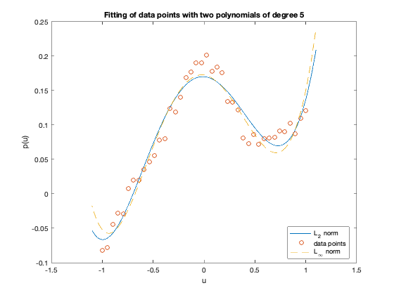
plot(u2, vpol,'-', u, v, 'o', u2, vpoll1,'--');
xlabel('u');
ylabel('p(u)');
title('Fitting of data points with two polynomials of degree 5');
legend('L_2 norm','data points','L_{\infty} norm', 'Location','Best');
% print -deps polapprox.eps
Computing optimal polynomial in the case of L2-norm...Done! 
Computing optimal polynomial in the case of Linfty-norm...Done!